average = mean =  = 6.0
= 6.0
--if all the values were the same in this dataset, what value would it be?
standard deviation =  = 2.30940108
--what is the amount of "scatter" around the average value?
--how should I round off this number? Significant digits...precision + 1
number = n = 10
--how many data points are there?
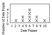
A histogram is most helpful in getting a "picture" of the data:

You might notice that these data fall into a sort of bell-shaped curve...a Gaussian curve. This is sometimes called a "normal" distribution. Not all data fall into a normal distribution. If data fit a normal distribution then about 68% of the data points are within 1 SD of the mean. 95% of the data points are within 2 SD of the mean. In the case of our simple data, 80% are within 1SD and 100% are within 2SD of the mean. Our sample is small and contrived! Larger datasets are more likely to fit a Gaussian distribution.
Data can also be graphed as a symbol at the mean, a box around the symbol extending +/- 1 SD, with lines extending over the range of data values:

Data Values
However data are shown, it is critical that the figure legend describe exactly what is being shown!! Don't forget legends on your figures! Label your graphs! Use a computer or at least a straightedge and graph paper!
If data fall into a normal distribution, we can use parametric statistical tests
(t, chi-square, regression, ANOVA, etc.)
If data do not fall into a normal distribution, we must go to non-parametric statistical tests.
(Wilcoxon, Kruskal-Wallis, etc.)
So let's say we have a second data set: 7,7,8,8,8,8,8,8,9,9  = 8.0 sd = 0.67
The averages are different, but the deviations encompass both averages. Are the two sets really different?
We first need a hypothesis. An educated guess about our question. We want to be able to reject it. Generally we are testing either a model for correctness, or a null-hypothesis (manipulation has no effect). SAMPLES ARE NOT DIFFERENT!
The parametric tests generally assume that the data sets are completely independent of each other, and are taken from a population distributed in a normal way (Gaussian). We need to check these assumptions out before starting!
The test we choose will go through some calculations that our friends, the statisticians have produced. Thank goodness computers can do all of this for us! In the old days we had to do the calculations by hand; the result was usually a value that had to be compared with a table of comparison values from a book. If your calculated value was above a certain table value you could reject your hypothesis. Your worksheet for this week provides the old-fashioned ways...but we will use the computer to see how to do the work more easily.
Nowadays, the computer can give us our old-fashioned values if we want them, but usually all you really need beyond the descriptive statistics, is the p-value. The p-value is the probability that the hypothesis you are testing accounts for the data observed. More accurately it is the probability that the differences between your data and the hypothesis are due to chance.
When p approaches 1.0 you become more sure of the hypothesis. As p approaches 0.0 you begin to have doubts or reject the hypothesis.
How low does p have to go before we reject the hypothesis? This is somewhat problematic...but the value that it must go below is called  . Convention sets alpha to 0.05, but this is a "one-size-fits-all" kind of value. It is good for some experiments, but is the wrong value for others. In other words, we allow 5% error in our testing. We are willing to be wrong one-time in twenty times...and still stick to our hypothesis!
What kind of errors are we talking about?
Statistical errors! NOT biology errors!
Type I: you reject a true null-hypothesis (convicting the innocent)
Type II: you fail to reject a false null-hypothesis (acquitting the guilty)
If you set  (reasonable doubt) too low, you will make lots of Type II errors, but will not make many Type I errors. Our justice system has been guilty of this.
If you set  (reasonable doubt) too high, you will make lots of Type I errors, but will not make many Type II errors. This is unthinkable in our justice system.
Screening pesticides: use a high  so that you don't miss any of the possibilities (Type I errors are OK...type II errors are fatal). Final pesticide testing for an virulent and otherwise untreatable pest, use a low
  to be sure that your pesticide beats nothing (Type II errors OK but want to avoid Type I)!
OK! Suppose your p-value is less than  . You can now reject the null-hypothesis. You can say your pesticide responses are statistically significant. But what if your p-value is very low? Is it more significant?
A test with p=0.001 is not more significant than a test with p=0.02 when your critical value is  =0.05; both are statistically significant. Many plant physiology articles will show numbers in tables with superscript symbols as found in the key below:
| symbol | p | meaning
|
|---|
| ns | >0.05 | not significant
|
| * | <0.05 | significant
|
| ** | <0.01 | very significant
|
| *** | <0.001 | extremely significant
|
Because of the various kinds of errors involved at different levels, you should not use these "meanings."
 = 6.0
= 6.0 = 2.30940108

 = 8.0 sd = 0.67
 . Convention sets alpha to 0.05, but this is a "one-size-fits-all" kind of value. It is good for some experiments, but is the wrong value for others. In other words, we allow 5% error in our testing. We are willing to be wrong one-time in twenty times...and still stick to our hypothesis!